LAB 4: Statistical Estimation

In this lab, we will examine:

• How to develop point estimates for population parameters
• The theory behind confidence intervals
• How to develop confidence intervals
• The 6 Steps for Calculating Confidence Intervals

Recommended web links:
Confidence Interval Applets: Experiment with confidence intervals and signficance levels.
 

Towards statistical inference...

The main goal of inferential statistics is to make inferences about population parameters based on sample data. There are two ways of making inferences about a population:

1. estimate the value of a population parameter using sample data
2. test a hypothesis about a population parameter or distribution using sample data.

Both methods reply upon probability and the sampling distribution theory that we explored in previous labs. In this lab, we will concentrate on estimation methods. In the next lab, we will examine hypothesis testing, which will form the basis for all subsequent statistical methods examined in this course.
 

There are two types of estimation procedures:

A. Point estimation

A single number, calculated from the sample data, is used as the best estimate of a population parameter. Point estimates can be developed for:

1. Population mean : There are several ways of estimating . You could use the median, the mode or the mean. However, if a sample is randomly selected from the population and has a normal frequency distribution, there is a high probability that the sample mean is close to the mean of the sampling distribution. The central limit theorem tells us that the mean of the sampling distribution equals the population mean . Therefore, is the best estimate of .

Example: In a study undertaken in Goldstream River, the mean stream velocity based on a sample of 25 measurements was found to be 10.8 m/sec. Therefore, 10.8 m/sec is our best estimate of the true stream velocity for the river.

2. Population proportion : The best estimate of a population proportion is the sample proportion, p, calculated from the sample.

Example: In a study of 200 commuters undertaken in Vancouver, the proportion (relative frequency) of commuters who travel by bus was found to be 128/200 = 0.64. Therefore, our best estimate of the proportion in the population, , is 0.64.
 

Point estimates are useful as they give us an estimated value for the parameter of interest (mean or proportion). We know that a statistic calculated from any one sample ( or p) will be close to the value of the population parameter ( or ). However, it is unlikely that a sample statistic will be identical to the population parameter and we may doubt the accuracy of our estimate. Therefore, it is useful to define a range or interval around our point estimate that is likely to include the population parameter.
 

B. Interval estimation

Two numbers define the interval within which the population parameter is thought to lie with a certain probability.

From Lab 3, we know that if we draw several different samples from the same population, the statistics calculated from each sample will differ. However, using information on probabilities and sampling distributions, we can specify an interval around our best estimate ( or p) so that there is a high probability that the population parameter lies within the interval. In other words, P(interval contains population parameter) = 0.95.

We will continue with the stream example from above where our best estimate of mean velocity was 10.8 m/sec.

Imagine that we place an interval of 2 m/sec around our estimate of mean velocity. This interval indicates that we believe the true mean stream velocity lies somewhere between 8.8 m/sec and 12.8 m/sec.

The sample of stream velocity contained 25 measurements. Imagine that we collect 9 additional samples, where each sample contains a different set of 25 velocity measurements. These 10 sample means will differ slightly, because each sample contains observations. We will place the 2 m/sec interval around each sample mean. The sample means and their associated intervals are outlined in the table below.

Sample	Sample mean (best estimate of )	Interval ( 2 m/sec)
A	10.8 m/sec	8.8 to 12.8 m/sec
B	9.0 m/sec	7.0 to 11.0 m/sec
C	11.9 m/sec	9.9 to 13.9 m/sec
D	13.5 m/sec	11.5 to 15.5 m/sec
E	8.4 m/sec	6.4 to 10.4 m/sec
F	10.4 m/sec	8.4 to 12.4 m/sec
G	8.1 m/sec	6.1 to 10.1 m/sec
H	10.3 m/sec	8.3 to 12.3 m/sec
I	9.3 m/sec	7.3 to 11.3 m/sec
J	11.5 m/sec	9.5 to 13.5 m/sec

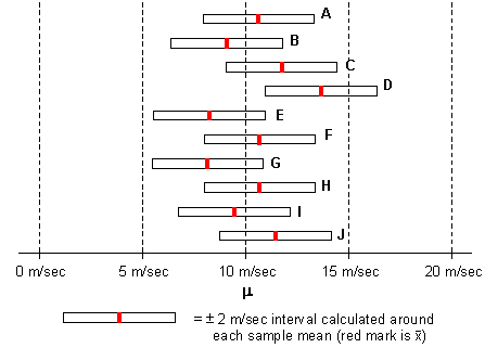
The diagram below shows the sample means and the intervals graphically. For the sake of this example, assume that we know the true mean stream velocity () is 10.0 m/sec. Notice that 9 of the intervals contain the true population mean. Only the interval for Sample D does not contain the true population mean.

If a sample mean is less than 8 m/sec or greater than 12 m/sec, the 2 m/sec interval around the mean will not contain the population mean. However, the probability that any sample mean is less than 8 m/sec or greater than 12 m/sec is fairly low. As we see in the diagram above, the 2 m/sec interval contains the population mean 9 times out of 10 (so the probability is 0.90).

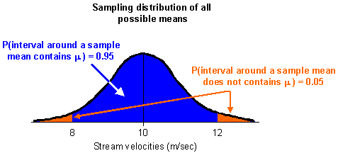
Imagine we drew 100 samples and found that the 2 m/sec interval around the means contains the population mean 95 times out of 100. We could say there is a 95% probability that the interval around a sample mean contains the population mean. If we drew all possible samples from this population, we may find that the probability that the 2 m/sec interval placed around each sample mean contains the population mean is also 0.95 (see the diagram below).

The probability value gives us a measure of confidence in the accuracy of our stream velocity estimate. With this interval, we can say "we estimate with 95% confidence that stream velocity in the Goldstream River is 10.8 m/sec 2 m/sec". We call this interval the confidence interval around our estimate.

In the example above, the size of the interval was given. In reality, you will not know how wide the interval should be. You could determine the size of the confidence interval by drawing all possible samples, plotting the sample means on a number line and finding the exact interval that contains 95% of the sample means. However, because we know that the sampling distribution of means follows the normal distribution (from the Central Limit Theorem), you can draw one sample and use a formula that incorporates Z scores to calculate a confidence interval around your best estimate.

Before we work with the formula, we need to examine the confidence interval probabilities more closely.
 

Confidence and Significance

Confidence intervals can be developed for any probability level:

P(interval contains parameter) = 0.80, 0.90, 0.95, 0.99 or even 0.99999.

• 0.90 (or 90%) is generally used for rough estimates
• 0.95 (or 95%) is the standard level used in most social science research
• 0.99 (or 99%) is often used in medical research where accuracy and high confidence in the estimate are extremely important.

These probabilities are called confidence levels and are expressed as (1 - ). The symbol (called 'alpha') refers to the probability that the parameter is outside the interval. When = 0.05, the confidence level is (1 - 0.05) = 0.95 or 95%. Alpha is also known as the significance level.

Significance Level ()		Confidence Level
0.10		(1 - 0.10) = 0.90 or 90%
0.05		(1 - 0.05) = 0.95 or 95%
0.01		(1 - 0.01) = 0.99 or 99%

When calculating a confidence interval, is evenly divided between the two sides of the sampling distribution. Therefore, the probability that the population mean is less than the confidence interval is divided by 2; the probability that the population mean is greater than the confidence interval is also /2.

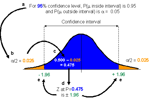
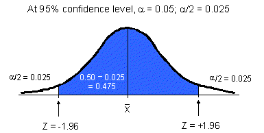
Since the sampling distribution has the same shape as a normal distribution, you can express the confidence level probabilities using a Z score (from the standard Z distribution). To do this, you need to find the value of Z that defines your confidence interval. The steps to finding Z for a 95% confidence interval are outlined below and in the accompanying diagram.

1. The confidence level is 95% so the probability that the parameter lies inside the interval is 0.95. The probability that the parameter lies outside the interval is = 0.05
    
   
2. is shared between both ends of the curve: /2 = 0.025
    
   
3. Because the Z distribution is symmetrical, you need only work with one side of the distribution. Therefore, we need to find Z at 0.500 - 0.025 = 0.475.
    
   
4. The Z value at P=0.475 is 1.96 (look up the probability in the Z table and work outwards to obtain the Z value).
    
   
5. Use - 1.96 and + 1.96 to define the appropriate confidence interval.
    
   

Probability and Sample Size

In the steps outlined above, we used the standard normal probability distribution (Z distribution) to model the probabilities in the sampling distribution. However, with a small sample, the probabilities associated with the Z distribution may underestimate the true variation in the population. For small samples, it is more appropriate to use the t-distribution. Therefore, we use the following rule when developing confidence intervals:

1. With a large sample (n > 30), you specify the confidence level probabilities using the Z distribution.
    
   
2. With a small sample (n < 30), you use the t-distribution to specify the confidence probabilities. In small samples, the standard deviation, s, may underestimate the true variation in the population. Therefore, there is a chance that your interval will be too narrow at a given confidence level. As the t-distribution is wider than the Z distribution for small values of n, it will compensate for this potential bias.

   The break between large and small samples ( 30) is not an absolute rule. It is a guideline or convention used by many statisticians. Any analyst could disregard the guidleline as long as he or she can provide a reasonable justification (e.g. you might use the t-distribution for a sample of n=35 because you want to be more conservative in your estimate).

Important note:
Confidence intervals should only be developed for variables with normal or approximately normal distributions. If the sample distribution is non-normal (highly skewed or bimodal), you should not calculate an interval.
 

Calculating Confidence Intervals

In this lab, we will calculate the following confidence intervals:

1. Confidence interval for a mean (based on a large sample)
2. Confidence interval for a proportion (based on a large sample)
3. Confidence interval for a mean (based on a small sample)
4. Special case: one-tailed confidence intervals

Note: In Lab 2, we started with an interval on the Z distribution and calculated the probability within the interval. In this lab, we start with a probability (or confidence level) and calculate the interval for this probability.

a) Confidence interval around a mean:

This formula is used to calculate confidence intervals (CI) for large samples:

Formula:

where: = sample mean (best estimate of ) = Z value associated with desired confidence level s = sample standard deviation n = sample size

Example: Calculate the 95% confidence interval for a sample (n=45) of tree heights, where = 24.5 m and s = 6.1 m.
 

1. As n is greater than 30, we will use the Z distribution for the confidence probabilities.
2. Find the appropriate Z value: At the 95% confidence level, = 0.05 and /2 = 0.025. Therefore, from the Z table, Z = 1.96.
   
   
   
3. Fill in the formula:
   

The confidence interval has a lower limit of 22.7 m (24.5 - 1.8) and an upper limit of 26.3 m (24.5 + 1.8). We estimate with 95% confidence that the true mean tree height is between 22.7 m and 26.3 m.
 

b) Confidence interval for a proportion:

The confidence intervals for proportions are constructed in a similar way to the intervals for means. The confidence intervals for proportions should only be calculated for very large samples (n>100). For smaller sample sizes, the sampling distribution of follows the binomial probability distribution (we are not covering this distribution in this course).

For a large sample, the formula is:

Formula:

where: p = sample proportion (best estimate of ) = Z value associated with desired confidence level n = sample size

Example: Calculate the 90% confidence interval for the proportion of teenage music customers who shop at ACME Music where p = 0.34 and n = 120 customers.
 

1. As n is larger than 100, we will use the Z distribution.
    
   
2. Find the Z value using the procedures outlined above.
   At 90% confidence level, = 0.10. Therefore, /2 = 0.05 and Z = 1.65.
    
   
3. Fill in the formula:
   

The confidence level has a lower limit of 0.27 (0.34 - 0.07) and an upper level of 0.41 (0.34 + 0.07). We estimate with 90% confidence that the true proportion of teenage customers who shop at ACME Music lies between 0.27 and 0.41.

c) Confidence interval for a mean (small sample):

The formula for small sample confidence intervals is:

Formula:

where: = sample mean (best estimate of ) = t value associated with desired confidence level & sample size s = sample standard deviation n = sample size v or df: degrees of freedom

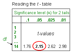
Example: Calculate the 95% confidence interval for a sample (n=15) of stream channel depths, where = 130 cm and s = 31 cm.
 


1. As n is less than 30, we use the t-distribution.
    
   
2. The method for determining the t value from the t-distribution table is different from that of the Z table.
   • The t values are specified for every combination of and df (degrees of freedom = n - 1).
      
     
   • is listed across the top. The t-table presents the significance level in a slightly different way. The table takes into account the fact that is divided between the two ends (or tails) of the distribution. So you look up the full under two tailed significance level on the t-table.
      
     
   • degrees of freedom (v or df) are listed down the side of the table.
      
     
   • To find your t-value:
     1. Determine : at the 95% confidence level, = 0.05
     2. Determine df: degrees of freedom (n - 1) = 14
     3. Use df=14 and the full = 0.05 to find t (see diagram below). In this case, t = 2.15.
     
     
3. Fill in the formula:
   

The confidence interval has a lower limit of 112.8 cm and an upper limit of 147.2 cm. We estimate with 95% confidence that the mean stream channel depth is between 112.8 cm and 147.2 cm.

d) One-tailed confidence intervals

The confidence intervals calculated above are considered two-tailed intervals as the probability covers both end (tails) of the distribution. This is the standard type of confidence interval. However, one-tailed confidence intervals (lower or upper limit) can be calculated if you are interested in a minimum or maximum value only.

Example: A car manufacturer states that mean carbon monoxide (CO) emissions for a given car model do not exceed 30 parts per million (ppm). A sample of 33 cars coming off the assembly line is taken determine if the car model meets the emission standards with 95% confidence. The sample statistics are: = 27.5 ppm and s = 5.3 ppm.

In this case, we are only interested in maximum emissions. Therefore, we will use an upper confidence limit to see if the mean car emissions are higher than the allowable level.
 


1. As n is greater than 30, we use the Z distribution.
    
   
2. As we are only interested in the upper tail of the distribution, the confidence probabilities are established as follows:
   1. The entire probability is allocated to the upper (right) side of the distribution. The interval covers all of the lower (left) side. At the 95% confidence level, = 0.05, so Z is +1.65.
       
      
   2. You can use any of the three confidence interval (CI) formulas for a one-tailed confidence bound. The difference in the formula is that for upper bounds, the calculated amount is added only; for lower bounds, the amount is subtracted only.
      

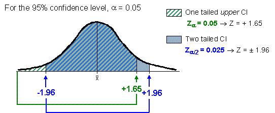
   This diagram shows the difference between a two-tailed confidence interval and a one-tailed upper confidence bound for the same confidence level:

   
   
3. Fill in the formula:
   

From this sample, we estimate with 95% confidence that the maximum mean carbon monoxide emission is 29.0 ppm; this car model (just) meets emission standards.

The 6 Steps for Calculating Confidence Intervals

1. Determine what kind of point estimate you are using:
   • mean
   • proportion
      
     
2. Select the appropriate probabilty distribution:
   • If mean and large sample (n > 30), use Z
   • If mean and small sample (n < 30), use t
   • If proportion and large sample (n > 100), use Z
      
     
3. Determine the appropriate or required confidence level:
   • 90%
   • 95% (standard confidence level)
   • 99%
   • other
      
     
4. Determine what kind of interval you need to calculate:
   • two-tailed
   • one-tailed (upper or lower)
     Read the question carefully and draw a quick sketch.
      
     
5. Determine the Z or t value (at or /2).
    
   
6. Calculate the interval or bound using the appropriate formula and present your results.

Remember that your confidence interval is based on one sample. There is a small probability (1%, 5%, etc.) that your sample mean or proportion actually falls at an extreme end of the sampling distribution. If you are using your confidence interval or estimate to recommend a course of action, it is often a good idea to take more samples to confirm the original estimate or inteval.

Example:
 
a. the cars in your sample exceed the carbon monoxide emission standards. Should you take more samples before recalling all cars of that model for emission repair?

OR

b. the cars in your sample just meet the emission standards. Do you believe these results (which are based on a single sample)? Should you take more samples to ensure the cars really do meet the standards?

Practice Questions

Q1. Complete the table below:

	Estimate	Interval type	Confidence level	n		Z or t?	Z or t value
A.		two tailed	90%	45
B.		two tailed	95%	12
C.		one tailed	95%	36
D.	p	two tailed	99%	180
E.		two tailed	80%	60
F.		one tailed	99%	23

Q2. Calculate the following confidence intervals:

1. Calculate a two-tailed 95% confidence interval around the estimate of mean length for a sample of 50 trout, = 35.6 cm and s = 9.4 cm.
    
   
2. Calculate a 90% confidence interval for the sample above.
    
   
3. In another sample of 200 trout, the proportion of fish over 4 years of age was 0.37. Calculate a two-tailed 95% confidence interval around this estimate.

Answers

Question 1

		Z or t?	Z or t value
A	0.10	Z	1.65
B	0.05	t	2.20
C	0.05	Z	1.65
D	0.01	Z	2.58
E	0.20	Z	1.28
F	0.01	t	2.51

Question 2:

1. 35.6 cm 2.6 cm. We estimate with 95% confidence that the true mean length lies between 33.0 cm and 38.2 cm.
    
   
2. 35.6 2.2 cm. We estimate with 90% confidence that the true mean length lies between 33.4 cm and 37.8 cm.
    
   
3. 0.37 0.07. We estimate with 95% confidence that the proportion of trout over 4 years of age lies between 0.30 and 0.44.