| |
In this lab, we will examine:
Recommended web links:
Hyperstat.com: A diagram of the
Chi-square distribution
VassarStats: An applet showing how
the Chi-square distribution changes with different degrees of freedom.
Enter degrees of freedom in the dialogue box that pops up (between 1 and 20)
Examples and Applications: An overview
and examples using the Chi-square distribution
There are two groups of inferential statistical tests: parametric and non-parametric tests. A parametric test requires that the underlying population for each sample is normally distributed, and that the data are either interval or ratio.
Non - parametric tests have been developed that use only frequency
counts in the calculation of the test statistics. No assumptions are made
about the shape of the underlying population distribution.
'Goodness of Fit' tests compare the frequencies observed in a sample to a distribution of expected frequencies in order to infer similarity.
When we discuss the mechanics of the non-parametric Goodness of Fit tests, you will notice the word distribution used in two different contexts.
| Shape of the 
|
| |
These tests use the hypothesis testing procedures detailed in Lab 5. For each test, we will outline:
The chi-square tests are the most basic tests because they use nominal categories and simple frequency counts. They are flexible tests because they can be applied to most data. However, these tests treat all categories as nominal so information associated with ordinal, interval or ratio levels of measurement will be lost.
In this discussion, we are going to start with one and two sample chi-square tests and then examine the one and two sample Kolmogorov-Smirnov tests.
This test uses the following statistical hypotheses:
| there is no difference between the observed and expected
frequencies (i.e. the sample is drawn from a population that follows the
expected distribution). | |
| there is a significant difference between the observed and expected frequencies (i.e. the sample is drawn from a population that does not follow the expected distribution). |
The test statistic provides a measure of the amount of difference between the
two frequency distributions. If the difference between the observed and expected
distributions is small, ![]() will be small. If the
difference is large,
will be small. If the
difference is large, ![]() will
be large.
will
be large.
Test Statistic
| Formula: | 
| where: Oi = observed frequency in each category Ei = expected frequency in each category |
|
Reject If the | 
|
 | 
|
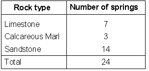
RESEARCH QUESTION: Is the occurrence of natural springs influenced by rock type?
1. Select the appropriate test:
To investigate this research question, we need to compare our observed frequencies
to a uniform frequency distribution. Why? If rock type is not important in determining
the location of springs, we will expect the number of springs to be evenly distributed
over rock type. If our observed frequencies are different from the expected
uniform frequencies, we can infer that rock type affects the occurrence of natural
springs. We will use the one sample chi-square test to answer our research question.
2. Check assumptions:
3. State your hypotheses:
4. Select significance level:
We will use the standard ![]() = 0.05 (95% confidence level)
= 0.05 (95% confidence level)
5. Select probability distribution of test statistic:
This test uses the ![]() distribution for the test
statistic
distribution for the test
statistic
6. Establish the critical values:
At ![]() = 0.05, and degrees of freedom (k-1) = 2,
the critical value (
= 0.05, and degrees of freedom (k-1) = 2,
the critical value (![]() ) = 5.99.
) = 5.99.
(Recall that k is the number of categories; we have 3 rock types so k = 3)
7. Calculate test statistic:
| Rock type | Observed frequency | Expected frequency | (Obs-Exp)2/Exp |
|---|---|---|---|
| Limestone | 7 | 8 | 0.13 |
| Calcareous Marl | 3 | 8 | 3.13 |
| Sandstone | 14 | 8 | 4.50 |
| Total | 24 | 7.75 |
Therefore, ![]() * = 7.75
* = 7.75
8. Make inference using the decision rule:
| Rule: reject From above, | 
|
9. State conclusion:
We conclude with 95% confidence that the observed frequencies are significantly
different from the expected (uniform) frequency distribution (i.e the springs
are not uniformly distributed between rock types). We infer that rock type influences
the occurrence of natural springs in Spring Valley.
| Rock type | Number of Springs |
|---|---|
| Limestone | 11 |
| Calcareous Marl | 5 |
| Sandstone | 14 |
| Volcanics | 6 |
| Total | 36 |
This test uses the following hypotheses:
If there are large differences between the observed and expected frequencies, the
![]() * test
statistic will be greater than the critical value. Therefore, we will reject
* test
statistic will be greater than the critical value. Therefore, we will reject
![]() and infer
that the samples are drawn from different underlying populations. If the differences between the
observed and expected frequencies are small,
and infer
that the samples are drawn from different underlying populations. If the differences between the
observed and expected frequencies are small, ![]() *
will be small and we will not reject
*
will be small and we will not reject ![]() . In this
case, we would infer that the samples are drawn from the same underlying population.
. In this
case, we would infer that the samples are drawn from the same underlying population.
| Formula: | 
| where: Oi,,j = observed frequency in each cell Ei,,j = expected frequency in each cell |
Note: the double ![]() means sum all rows and columns in the table.
means sum all rows and columns in the table.
RESEARCH QUESTION: Is there a significant difference between the responses of the user groups?
| Reponses | Samples (user groups) | Row Totals | ||
|---|---|---|---|---|
| Daily Commuters | Commercial Operators | Tourists | ||
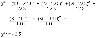
| Widen | 19 | 22 | 26 | 67 |
| Tunnel | 8 | 35 | 14 | 57 |
| Transit | 33 | 3 | 20 | 56 |
| Column Totals | 60 | 60 | 60 | 180 |
1. Select the appropriate test:
We need to determine if there are differences between the observed frequencies
of 3 samples (user groups). If the responses of the user groups are similar
we can infer that the user groups are all part of the same underlying population.
If there are differences in the responses, we can infer that the user groups
come from different parent populations. We will use the multi-sample ![]() test
test
2. Check assumptions:
Each cell in the table is referenced as follows:

For each cell, the expected frequency (at row I and column J) is:
![]()
For our data, the expected frequencies are:
Daily / widen bridge: E1,1 = (67 * 60)/180 = 22.3
Commercial / widen bridge: E1,2 = (67 * 60)/180 = 22.3
...
Commercial / tunnel: E2,2 = (57 * 60)/180 = 19.0
...
Tourist / transit: E3,3 = (56 * 60)/180 = 18.7
The observed and expected frequencies are shown in this table:
| Responses | Commuters | Operators | Tourists | Total | |||
|---|---|---|---|---|---|---|---|
| Obs | Exp | Obs | Exp | Obs | Exp | ||
| Widen | 19 | 22.3 | 22 | 22.3 | 26 | 22.3 | 67 |
| Tunnel | 8 | 19.0 | 35 | 19.0 | 14 | 19.0 | 57 |
| Transit | 33 | 18.7 | 3 | 18.7 | 20 | 18.7 | 56 |
| Total | 60 | 60 | 60 | 180 | |||
No expected frequency is less than 5
![]() we can apply this test.
we can apply this test.
3. State your hypotheses:
4. Select significance level:
We will use standard ![]() = 0.05 (95% confidence level)
= 0.05 (95% confidence level)
5. Select probability distribution of test statistic:
This test uses the
![]() distribution for the test statistic.
distribution for the test statistic.
6. Identify the critical values:
At ![]() = 0.05, degrees of freedom (k-1)*(l -1) =
(3-1)*(3-1) = 4, therefore
= 0.05, degrees of freedom (k-1)*(l -1) =
(3-1)*(3-1) = 4, therefore ![]() = 9.49. (Recall
that k is the number of categories and l is the number of samples)
= 9.49. (Recall
that k is the number of categories and l is the number of samples)
7. Calculate test statistic:
|
8. Compare using the decision rule:
| Rule: reject From above, | 
|
9. State conclusion:
We infer with 95% confidence that there is a significant difference between the responses of
the user groups in terms of their preferences of alternatives for the Lions Gate Bridge
crossing.
| Case | Obs | Exp | Difference | Comments |
|---|---|---|---|---|
| A | 510 | 500 | 10 | These frequencies are quite large, so the difference of 10 is relatively minor. |
| B | 10 | 5 | 5 | These frequencies are small, so the difference of 5 is very important. The observed frequency is twice as large as the expected. |
In the hypothesis test, you would probably reject ![]() in case A (and infer a significant difference) and not reject
in case A (and infer a significant difference) and not reject ![]() in case B (and infer no difference). Because the critical value
(
in case B (and infer no difference). Because the critical value
(![]() ) is based on number of categories and
not sample size, the test cannot account for the relative differences in actual frequencies.
) is based on number of categories and
not sample size, the test cannot account for the relative differences in actual frequencies.
Although there are limitations to the chi-square, these tests are easy to use and have
many applications, particularly for analyzing survey or social data. In these types of
research, the data are usually collected at the nominal scale.
The Kolmogorov-Smirnov (KS) tests also compare observed and expected frequencies. However, these tests are different from the chi-square tests because the KS tests use cumulative relative frequencies in their test statistic. To develop cumulative relative frequencies, the data must be at the ordinal scale. These tests are considered more powerful that the chi-square tests because they use a higher level of measurement. However, the ordinal scale restriction means that the tests cannot be applied as widely as the chi-square tests.
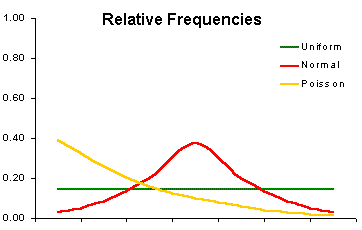
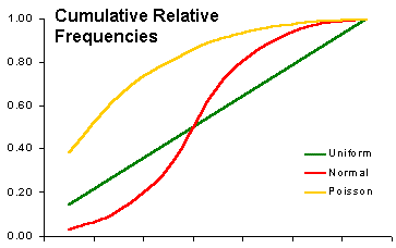
| Three ways to display frequencies |
|---|

|
| Comparing 3 expected distributions |
|---|
|
This test compares the two cumulative relative frequencies (CRF) to find the maximum difference between the observed and expected frequencies. The maximum difference is the D* test statistic.
| Observed CRF vs 3 Expected CRF |
|---|

|
| Note: for this example, the observed frequencies have an approximately normal shape with a slight negative skew. Therefore, there is only a small difference between the observed and expected (normal) frequencies. |
This test uses the following hypotheses:
| there is no difference between the observed and expected frequencies
(i.e. the sample is drawn from a population that follows the expected
distribution). | |
| there is a significant difference between the observed and expected frequencies (i.e. the sample is drawn from a population that does note follow the expected distribution). |
If the two cumulative relative frequencies are similar, the maximum difference (D) will be
small and we cannot reject ![]() . We infer that the
observed distribution follows the expected distribution. If, however, there is a large
difference between the two cumulative relative frequencies (D is large), we reject
. We infer that the
observed distribution follows the expected distribution. If, however, there is a large
difference between the two cumulative relative frequencies (D is large), we reject ![]() .
.
| Formula: | |
| this means "D* is the maximum (or largest) absolute (without + or - sign) difference
between the observed cumulative relative frequencies ( |
QUESTION: Are her data normally distributed?
| Persons per household | Observed Frequency |
|---|---|
| 1 to 2 | 3 |
| 3 to 4 | 5 |
| 5 to 6 | 6 |
| 7 to 8 | 9 |
| 9 to10 | 15 |
| 11 to12 | 23 |
| 13 to14 | 9 |
| Total | 70 |
Note: For this problem, the expected frequencies based on the normal distribution are printed for you, but see note below on computing expected normal distribution.
1. Select appropriate test:
We will use the one sample KS test because it will allow us to compare the observed
frequencies against the frequencies expected for a normal distribution. This
test also allows us to retain the ordinal nature of the data (a chi-square test
would convert the ordinal categories to nominal categories, resulting in a loss
of information).
2. Check assumptions:
3. State your hypotheses:
4. Select the significance level:
We will use the standard ![]() = 0.05 (95% confidence
level)
= 0.05 (95% confidence
level)
5. Establish the probability distribution of the test statistic:
Because we are conducting a KS test, we use the D distribution for the test
statistic.
6. Establish the critical values:
At ![]() = 0.05, degrees of freedom (n) = 70,
= 0.05, degrees of freedom (n) = 70, ![]() = 0.16
= 0.16
7. Calculate the test statistic:
| Category | Observed | Expected | D | ||||
|---|---|---|---|---|---|---|---|
| 1-2 | 3 | 3 | 0.04 | 2 | 2 | 0.03 | 0.01 |
| 3-4 | 5 | 8 | 0.11 | 7 | 9 | 0.13 | 0.02 |
| 5-6 | 6 | 14 | 0.20 | 13 | 22 | 0.31 | 0.11 |
| 7-8 | 9 | 23 | 0.33 | 26 | 48 | 0.69 | 0.36 |
| 9-10 | 15 | 38 | 0.54 | 13 | 61 | 0.87 | 0.33 |
| 11-12 | 23 | 61 | 0.87 | 7 | 68 | 0.97 | 0.10 |
| 13-14 | 9 | 70 | 1.00 | 2 | 70 | 1.00 | 0.00 |
| Total | 70 | 70 | |||||
From the table, D* is 0.36
8. Make inference using the decision rule:
9. State conclusion:
We conclude with 95% confidence the observed frequencies are significantly different
from the expected (normal) frequency distribution. Therefore, we infer that
the underlying population is not normally distributed and the researcher cannot
use parametric tests to analyse these data.
Rejecting ![]() follows the same
logic given in the one-sample KS test.
follows the same
logic given in the one-sample KS test.
| Formula: | |
| "D* is the maximum absolute difference between the CRF in sample A and
the CRF in sample B" |
| Significance Level ( | Critical D formula |
|---|---|
| 0.10 | 1.22 * |
| 0.05 | 1.36 * |
| 0.025 | 1.48 * |
| 0.01 | 1.63 * |
| 0.005 | 1.73 * |
| 0.001 | 1.95 * |
A regional planner is reviewing the proposed expansion of recreational facilities for two communities. The age structure of each community will influence the type of new or expanded facilities (i.e. daycare and children’s programs or seniors’ activity center). In the past, the two communities had similar demographics. However, recent migration trends may have changed the demographic patterns. Random sampling was conducted in each community; the data are presented below.
| Age classes | Port Francis | Pebble Beach |
|---|---|---|
| 0-10 | 59 | 31 |
| 11-18 | 53 | 37 |
| 19-44 | 48 | 45 |
| 45-64 | 32 | 57 |
| 65+ | 18 | 35 |
| Total | 210 | 205 |
RESEARCH QUESTION: Is there a significant difference between the age classes
of the two communities? Check your answer.
To use this distribution, the data must fulfill certain conditions:
Calculating Poisson frequencies is a two step process. The steps are outlined below. Then we will apply these steps to calculate Poisson frequencies for lightning stikes.
Step 1: Calculate the average number of events (![]() )
per unit area or block of time
)
per unit area or block of time
Step 2: Use ![]() to calculate the
expected Poisson frequencies:
to calculate the
expected Poisson frequencies:
| Formula: | 
| where x = number of events per time period or unit of space e = 2.71828 (base or natural logarithm) |
Example: The number of lightning strikes per day were recorded in Alberta for 6 summers (for months of July and August). The data are presented below.
| Strikes per day | Days | 
|
|---|---|---|
| 0 | 209 | |
| 1 | 115 | |
| 2 | 32 | |
| 3 | 8 | |
| 4 | 1 | |
| Total | 365 |
| Strikes per day (Xi) | Days (w) | # of strikes |
|---|---|---|
| 0 | 209 | 0 * 209 = 0 |
| 1 | 115 | 1 * 115= 115 |
| 2 | 32 | 2 * 32 = 64 |
| 3 | 8 | 3 * 8 = 24 |
| 4 | 1 | 4 * 1 = 4 |
| Total | 365 | 207 |
![]() = 207/365 = 0.567 strikes per day
= 207/365 = 0.567 strikes per day

To develop the Poisson frequency distribution, you will perform the same calculation for each category of lightning strikes. Two calculations and the completed table of expected frequencies are shown below.
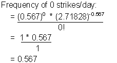 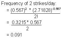
|
*Note: due to rounding, may not add to 1. |
For a one sample KS test, the frequencies we calculated above would
be used to develop the expected cumulative relative frequencies. The table below
shows ![]() and
and ![]() for the KS test.
for the KS test.
| Category (strikes per day) | Observed frequency (days) | Expected Frequency (days) | D | |||
|---|---|---|---|---|---|---|
| 0 | 209 | 207 | 209 | 0.573 | 0.567 | 0.006 |
| 1 | 115 | 118 | 324 | 0.888 | 0.889 | 0.001 |
| 2 | 32 | 33 | 356 | 0.975 | 0.980 | 0.005 |
| 3 | 8 | 6 | 364 | 0.997 | 0.997 | 0.000 |
| 4 | 1 | .73 | 365 | 1.000 | 1.000 | 0.000 |
| Total | 365 | 364.73 |
We can see that the cumulative relative frequencies of lightning strikes observed in Alberta are very similar to the frequencies expected in a Poisson distribution. A significance test would confirm that the observed frequencies are not different from the Poisson distribution. Conduct the test and prove it for yourself (check your answer).
| Rock type | Observed | Expected | (Obs-Exp)2/Exp |
|---|---|---|---|
| Limestone | 11 | 9 | 0.44 |
| Calcareous Marl | 5 | 9 | 1.78 |
| Sandstone | 14 | 9 | 2.78 |
| Volcanics | 6 | 9 | 1.00 |
| Total | 36 | 6.00 |
Decision:
Rule: reject ![]() if
if ![]() *
>
*
> ![]()
![]() * (6.00) is less than
* (6.00) is less than ![]() (7.82), so we cannot reject
(7.82), so we cannot reject ![]() (we conclude with 95% confidence that the sample is drawn from a population
that is significantly different from uniform).
(we conclude with 95% confidence that the sample is drawn from a population
that is significantly different from uniform).
Critical values:
At ![]() = 0.05,
= 0.05,

Test statistic:
D* is shown in red.
| Age Class | Port Francis | CFA | CRFA | Pebble Beach | CFB | CRFB | D |
|---|---|---|---|---|---|---|---|
| 0-10 | 59 | 59 | 0.28 | 31 | 31 | 0.15 | 0.13 |
| 11-18 | 53 | 112 | 0.53 | 37 | 68 | 0.33 | 0.20 |
| 19-44 | 48 | 160 | 0.76 | 45 | 113 | 0.55 | 0.21 |
| 45-64 | 32 | 192 | 0.91 | 57 | 170 | 0.83 | 0.08 |
| 65+ | 18 | 210 | 1.00 | 35 | 205 | 1.00 | 0.00 |
| Total | 210 | 205 | |||||
Decision:
Rule: reject ![]() if D* >
if D* > ![]()
From above, D* (0.21) is greater than ![]() (0.13), so we can reject
(0.13), so we can reject ![]() (we
conclude with 95% confidence that the two samples are drawn from significantly
different underyling populations).
(we
conclude with 95% confidence that the two samples are drawn from significantly
different underyling populations).
Critical value:
At ![]() = 0.05 and degrees of freedom (n = 365),
we use the formulas at the bottom of the critical D table to compute the critical
value.
= 0.05 and degrees of freedom (n = 365),
we use the formulas at the bottom of the critical D table to compute the critical
value. ![]() = 0.071.
= 0.071.
Test statistic:
From the lightening strike example, we found that D* was 0.006.
Decision:
Rule: reject ![]() if D* >
if D* > ![]()
From above, D* (0.006) is less than ![]() (0.071), so we cannot reject
(0.071), so we cannot reject ![]() (we conclude with 95% confidence that the sample is drawn from a population
that is not different from expected - the observed distribution follows the
Poisson distribution)
(we conclude with 95% confidence that the sample is drawn from a population
that is not different from expected - the observed distribution follows the
Poisson distribution)
| © University of Victoria
2000-2001 Geography 226 - Lab 6 Developed by S. Adams and M. Flaherty Updated: September 30, 2001 |