|
|
In this lab, we will examine:
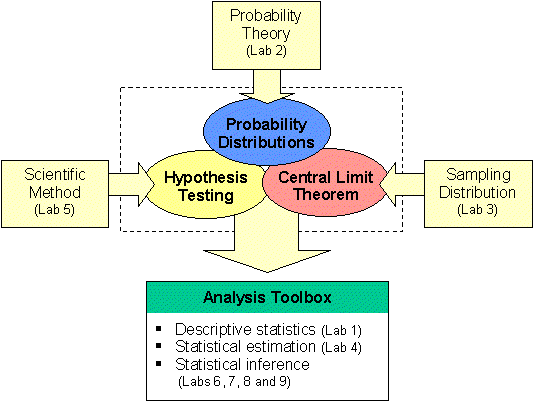
Probability is a fundamental building block for inferential statistics. Inferential analyses use probability theory to make confidence statements about the characteristics of populations based on sample information, or to test hypotheses. The diagram below is a road map to building the Analysis Toolbox. We have already covered one component of the toolbox - descriptive statistics. Before we can consider methods for statistical estimation and inference, we must navigate through probability distributions (this lab), sampling and the central limit theorem (Lab 3), and later hypothesis testing (Lab 5).
| Road Map to the Analysis Toolbox |
|---|
|
We encounter probability statements on an almost daily basis. They are used to express the chance of rain, the likelihood of winning the lottery, or the chance of a major earthquake on Vancouver Island (which is higher than we would all like to believe!). In considering probability statements, it is important to remember that probabilities can be obtained in different ways. Some probabilities are purely subjective and are based on 'gut feeling' or 'best guess.' These are not the concern of this course. We will focus on probablities that are either based on observation or derived from theory.
Probabilities provide a quantitative description of the likely occurrence of a particular event, and are expressed on a scale from 0 to 1 (or 0 to 100%). A rare event has a probability of occurance close to 0, while a very common event has a probability of occurance close to 1.
A common way of obtaining probabilities is from data. The probability of an event occurring, written as P(E), is defined as the proportion of times the event occurs in a series of trials.
Example: to assess the probability of rain on a given day in Victoria between November and February, you could record each day of rain during this period, and calculate the proportion of rainy days relative to the total number of days:

Conclusion: On any given day in winter, the probability of rain is 0.73 or
73% (yuk!). The probability of a sunny day during this period is 1 - 0.73 =
0.27.
We can also calculate probabilities without having to directly observe the frequencies.
Example: In a valley, there are 7 tree species and 15 plant species; 2 tree and 5 plants species are non-native (introduced). What is the probability that a species selected at random is non-native?
What is the probability that a tree species is introduced?
Example: what is the probability of rolling a '3' on a six-sided die?
In section A above, we dealt with one event (weather) that had 2 possible outcomes (rain or sun). You can also calculate probabilities for multiple events, each with different outcomes. Consider the weather (Event A) and taking a bus (Event B). Event A has two outcomes; Event B has three outcomes (the bus is early, on time, or late). You may want to know if the probability that the bus is late increases when it rains.
It is helpful to use a diagram to visualize the events (solid boxes) and outcomes (dashed boxes):

|
An important consideration for multiple events is whether they are independent or dependent. Two events are independent if the probability of one occurring does not affect the probability of the other. With dependent events, the probability of one event affects the chances of the other occurring.
Consider this: lack of sleep can adversely affect our reaction times, particularly
when driving. Since the majority of drivers have not had a severe accident,
it is reasonable to assume that the ‘average’ probability of having a severe
accident is low. However, if a person is sleep- deprived, the probability of
a severe accident could increase dramatically. In the latter case, the probability
of having a severe accident depends on the probability that a person
has slept well or not.
In the weather/bus example, the probability that a bus is late may depend partly on the weather. When it rains, there may be a higher probability that the bus is late because the bus driver drives more slowly in the rain or because more people take the bus. However, if the bus had the same probability of being late, regardless of the weather, we could say these two events are independent.
There are 4 rules that allow you calculate more complex probabilities.
RULE 1: Adding Probabilities (OR)
For mutually exclusive outcomes within a single event (outcomes that do not occur at the same time), you add the individual outcome probabilities; Outcome A OR Outcome B OR Outcome C.
Example: As a transit planner, you are evaluating the time allocation for a bus schedule during rush hour. You observe that the bus is early 20% of the time and late 35% of the time. What is the probability that the bus is early or late?
| P(early OR late) |
= P(early) + P(late) = 0.20 + 0.35 = 0.55 | 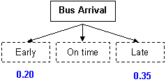
|
| The probability that the bus is early or late = 0.55. | ||
RULE 2: Complementary Probabilities (NOT)
Because the outcome probabilities in one event will sum to 1, you can calculate the probability of an outcome NOT occurring. What is the probability that the bus will arrive on time (not early or not late)?
| P(NOT early or NOT late) |
= 1 - P(early OR late) = 1 - 0.55 = 0.45 | 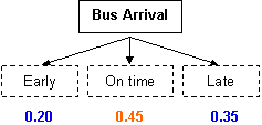
|
| The probability that the bus arrives on time = 0.45. | ||
RULE 3: Multiplying Probabilities (AND)
a) For outcomes within a single event, you multiply the individual outcome probabilities; Outcome A AND Outcome B AND Outcome C.
Example: What is the probability that the bus will be late twice in a row?
| P(late AND late) |
= P(late) * P(late) = 0.35 * 0.35 = 0.12 | 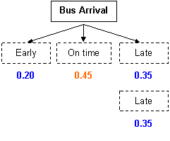
|
| The probability that the bus is late twice in a row = 0.12. | ||
b) For outcomes of multiple independent events, you can also multiply the probabilities; Outcome 1 for Event A AND Outcome 1 for Event B
Example: The bus service under study takes passengers to the ferry. The ferry departs late 40% of the time regardless of the bus arrival. Therefore, these two events are independent. What is the probability that the bus is late AND the ferry is late?

|
NOTE: you cannot use the straight multiplication formula when the events are dependent. When events are dependent, the probabilities associated with outcomes for one event are based on the outcome probabilities of a previous event. In this case, you must use conditional probabilities.
RULE 4: Conditional Probability
Whenever events are dependent on each other, the probabilities are referred to as conditional and are calculated from a joint probability table. Returning to the sleep and driving example above, the following data were collected from 200 vehicle accidents:
To calculate conditional probabilities, the raw data must be transformed into a joint probability table.
| Lack of sleep | Enough sleep | Total | |
| Minor accident | 0.61 | 0.20 | 0.81 |
| Severe accidents | 0.17 | 0.02 | 0.19 |
| Total | 0.78 | 0.22 | 1.00 |
Step 3: What is the probability of a severe accident given that the driver is sleep deprived?
| P(severe accident | lack of sleep) | = P(severe accident
AND lack of sleep) P(lack of sleep) |
| = 0.17/0.78 = 0.22 |
The probability that a sleep-deprived driver has a severe accident is 0.22 or 22% (compared to 9% for well-rested drivers).
Note that the symbol " | " is used for the word "given". In the example above,
P(severe accident | lack of sleep) is read as "the probability of a severe
accident given that the driver has a lack of sleep".
A probability distribution lists the possible outcomes within an event and the probabilities associated with each outcome. For a given variable, there is a probability associated with each possible value.
|
Example: this graph shows the probability distribution for bus arrivals, based on the probabilities discussed above. | 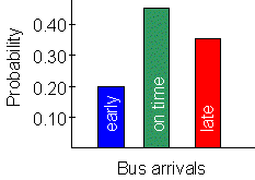
|
You can also create probablity distributions for other variables, such as height, weight, carbon dioxide concentrations, etc,.
|
Example: this graph shows the probabilty distribution for the sample of heights discussed in Lab 1. There were 17 people out of 30 with heights between 170 and 179 cm. Therefore, the probability that any person is 170 to 179 cm tall is 0.57. If this sample had 10,000 observations, the distribution would become more smooth and take on a curved shape - similar to the normal curve. | 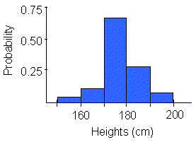
|
There are several different probability distributions because there are different types of events and populations. In lab 1, we observed that the pattern of heights followed a normal distribution. Therefore, we would use the normal probability distribution to model this population.
However, there are cases where the normal distribution cannot be used to model a phenomenon. For example, the number of lightening strikes in a day is not normally distributed. You would expect many days without any strikes, a few days with one strike, and very few days with multiple strikes. These discrete rare events can be modeled using the Poisson probability distribution which we will consider in later labs. Two common probability distributions are outlined in the next section.
The characteristics of the normal probability distribution are:
You can define intervals around the mean based on the standard deviation. Approximately
68% of values fall within ![]() 1 standard deviation
of the mean. You can also define larger intervals around the mean based on 2
standard deviations or 3 standard deviations.
1 standard deviation
of the mean. You can also define larger intervals around the mean based on 2
standard deviations or 3 standard deviations.
Example: If ![]() = 145 cm and s =
= 145 cm and s =
![]() 5 cm , then 2 s =
5 cm , then 2 s = ![]() 10 cm, and 3 s =
10 cm, and 3 s =
![]() 15 cm.
15 cm.
Careful study of normal distributions has shown that approximately 95% of observations
lie within ![]() 2 standard deviations of the mean and
approximately 99.7% of observations lie within
2 standard deviations of the mean and
approximately 99.7% of observations lie within ![]() 3 standard deviations of the mean.
3 standard deviations of the mean.

|
What does this mean? In the example above, 99.7% of all observations in the sample will fall between 130 cm and 160 cm (within the interval defined by 3 standard deviations). This means you know the probability that any observation is less than 130 cm or bigger than 160 cm is very low (this probability is 0.003 or 0.3%).
What is the probability that any observation in the sample is less than the mean (145 cm)? Using the diagram above, you can calculate this probability:
What is the probability that any observation is greater than 150 cm? To determine this probability, locate 150 cm on the diagram. It lies at the upper end of the 2 s interval. Therefore,
Note that all probabilities under the normal curve add to 1.0 or 100%.
The above probabilities were relatively easy to calculate because we were using
the probabilities for the standard deviation intervals. What if you want to
calculate a probability that is not exactly defined by a standard deviation
interval? For example, you want to calculate the probability that any value
is greater than 147 cm. How will you do this?
There is a formula for calculating probabilities under the normal curve from
raw data, but it is very cumbersome. Fortunately, statisticians have developed
a standard normal probability distribution in units of Z. This standard
distribution has a mean of 0 z and a standard deviation of
![]() 1 z. The probabilities associated with every Z value have been calculated and
are presented in a table.
1 z. The probabilities associated with every Z value have been calculated and
are presented in a table.
The diagram below shows the standard normal probability distribution (or Z distribution), with the standard deviation intervals in terms of Z.
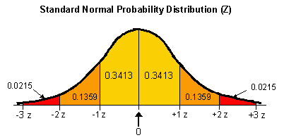
To determine specific probabilities, you convert your raw data into Z values. Using Z values, you can calculate probabilities based on the area under the curve. You can then convert the probabilities back into values, if necessary.
For the following applications, we will consider a sample of gasoline prices
(¢ per litre) in the city of Victoria where
![]() = 65.4¢ and s = 3.9¢.
= 65.4¢ and s = 3.9¢.
Click
here to refer to online normal distribution or z-score table
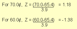
Q 1: What is the probability that a litre of gas costs between 60¢ and 70¢?

|
| Formula: | 
| where xi = a specific value or any value in the dataset s = standard deviation |
| ||
Note: Z tables usually state the area under the curve (probability) from
the mean (0) to Z for one side of the distribution. (Look at the drawing at
the top of the Z table so you know which probabilties are shown in the table).
If your interval covers both sides of the distribution, add the probability
for the positive and negative sides of the Z distribution.
P(0 to 1.18) = 0.3810
P(0 to -1.38) = 0.4162
P(-1.38 to 1.18) = 0.4162 + 0.3810 = 0.7972
There is a 0.797 or 79.7% probability that gas prices range between 60¢
and 70¢.
Always check your results against your sketch to confirm your calculations.
In this case, the orange portion seems to account for about three-quarters
of the area under the curve. Therefore, our probability of 0.797 is likely
to be correct.

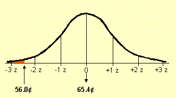
Q 2: What is the probability that gas prices will fall below 56¢?
|
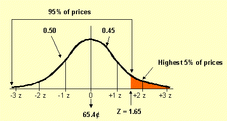
Q 3: How expensive are the highest 5% of gas prices?
This question starts with a probability and works backward to obtain a value. This is the opposite of Q1 and Q2.
|
| Formula: | where: Z = Z value s = standard deviation |
You can use the calculated probabilities to answer more questions:
Q 4: In the next 6 months, how many days will gas cost 56¢ or less?
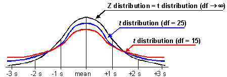
Important note on the Z distribution:
If you add all the probabilities between - 2z and + 2z, you will notice that
they sum to slightly more than 0.95. In fact, the sum of probabilties between
![]() 2z is:
2z is:

|
|