| |
In the lab, we will examine important concepts of regression analysis, including:
Recommended Web Links:
Regression applets from the
University of Illinois and
David Howell
Regression is a complex but extremely useful statistical procedure that has
applications in many areas of geography: social, economic, physical, geomatics,
etc. As with any tool, regression analysis has several limitations, which a
researcher must understand in order to apply it appropriately. In this lab,
we will explore the fundamental concepts of regression, and then work through
the application of regression analysis using an example.
In lab 8, we used correlation to assess the degree of linear association between two variables, in terms of direction and strength of the relationship. It was stressed, however, that a strong correlation did not imply the existence of a causal relationship between the variables.
Causal relationships do exist in nature. For example, the amount of runoff is related to the amount of rainfall in a watershed. Heavy rainfall causes more runoff; low rainfall causes less runoff. A geographer could use this information to predict runoff based on their knowledge of rainfall in the watershed. In order to apply regression analysis, it is necessary to assume a causal (or 'functional') relationship between two variables. A researcher can then develop an equation useful for prediction.
| This distinction very important as the results
of the analysis depend on how you specify your variables. In our watershed
example, rainfall is the independent variable and runoff is the dependent
variable. Rainfall will influence the amount of runoff, but runoff will
have no effect on the amount of rainfall.
The convention in regression is to label your independent variable as X and your dependent variable as Y. This convention extends to scatter plots where the independent variable is plotted along the X-axis and the dependent along the Y-axis. | 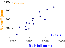
|
A functional relationship is often stated as "Y is a function of X". Using
the rainfall example, we would say that "runoff is a function of rainfall".
The short hand version of this statement uses the symbol 'f()' which stands
for "function of". Therefore, we would write: runoff = f(rainfall). This format
is very useful when you have multiple variables that may be causing an effect.
For example: runoff = f(rainfall, soil storage, plant intake). In this course,
we will only consider simple linear (or bivariate) regression with one independent
variable.
To estimate runoff based on rainfall, we need an equation that relates the values of one variable (rainfall) to values of the other (runoff). Examples of equations may include:
How would you develop an equation between these two variables? You could develop an approximate relationship by looking at the data (see the table below).
The data for rainfall and runoff are presenting in the table below. For example, we could use the data in the first row (rainfall = 1842, runoff = 1156) to develop the equation: runoff = 0.628*rainfall.
We can test this equation by applying it to all other rows (Prediction) and calculating the difference between the observed and estimated value (Error). We find our equation gives small error for three cases and large errors for the rest. We conclude that this equation does not accurately predict runoff based on rainfall.
| Rainfall | Runoff | Prediction | Error |
|---|---|---|---|
| 1842 | 1156 | 1155 | 1 |
| 2202 | 1378 | 1381 | -3 |
| 2036 | 1274 | 1277 | -3 |
| 1868 | 947 | 1171 | -224 |
| 1520 | 356 | 953 | -597 |
| 1350 | 454 | 846 | -392 |
| 1710 | 610 | 1072 | -462 |
| 1510 | 473 | 947 | -474 |
| 1285 | 127 | 806 | -679 |
| 1522 | 651 | 954 | -303 |
| 1585 | 380 | 994 | -614 |
| 1682 | 750 | 1055 | -305 |
| 1984 | 820 | 1244 | -424 |
| 1594 | 641 | 999 | -358 |
| 1693 | 850 | 1062 | -212 |
You could try developing an equation from data in the 5th row or the 10th row or... However, the data in each individual row may not accurately represent the 'overall' relationship between the two variables, and you end up with large errors. What you really want is an equation that minimizes the overall error (the differences between observed and predicted value). This equation may not exactly predict each observed value, but it will give you results that are close for most cases.
| One way to develop this equation is to prepare a scatter plot and draw a straight line through the points. This straight line should be as close as possible to each point (but you can't play 'connect the dots'!). There are many lines you could draw (in blue), but only one line will minimize the overall error for all points. This is called the Line of Best Fit (in red). | 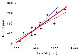
|
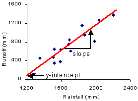
This line will have a specific equation,
based on:
| 
|
The slope and y-intercept are expressed in algebra in the regression model:
| where: Y = the dependent variable (runoff) X = the independent variable (rainfall) |
SPSS will calculate the values for ![]() and
and ![]() for you. Finding the line
of best fit by hand would be an extremely long and slow process, which is why
regression was not used in research until recently. Today, computers can do
the necessary calculations in a few seconds.
for you. Finding the line
of best fit by hand would be an extremely long and slow process, which is why
regression was not used in research until recently. Today, computers can do
the necessary calculations in a few seconds.
How does the computer find the line of best fit?
| Most statistical software packages use a
procedure called Ordinary Least Squares (OLS) to find the
line of best fit. This procedure evaluates the difference (or error) between
each observed value and the corresponding value on the line of best fit.
We use vertical distance as our measure of error because we are interested
in how close our predicted answer ( Note: The errors are squared to remove the + or - sign. If the + and - signs are not removed, the positive errors can cancel out the negative errors, which could give you a value of zero. | 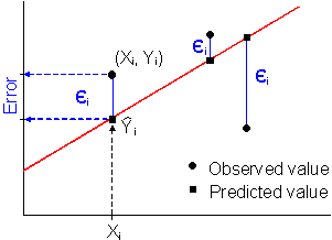
|
Once we have obtained the value of ![]() and
and ![]() for the line of best fit, we need to assess how well the line fits the original
data. In particular, we want to know how well the independent variable (X) explains
or accounts for the variation in the dependent variable (Y). If X explains most
of the variation in Y, we infer that the line fits the data well. Another consideration
is that we need to have a measure that does not depend on the scale or units
of the variables; this would allow us to compare the results of different regression
analyses.
for the line of best fit, we need to assess how well the line fits the original
data. In particular, we want to know how well the independent variable (X) explains
or accounts for the variation in the dependent variable (Y). If X explains most
of the variation in Y, we infer that the line fits the data well. Another consideration
is that we need to have a measure that does not depend on the scale or units
of the variables; this would allow us to compare the results of different regression
analyses.
To evaluate how much of the variation in Y that X explains, we need a baseline
for comparison. If X had no effect on Y, our best estimate for Y is the mean
(![]() ). Therefore, the difference
between
). Therefore, the difference
between ![]() (observed) and
(observed) and ![]() (mean) is our baseline for comparison. This difference is called the total
variation. Then we can compare the variation explained by X to the total
variation to quantify how much effect X has on Y.
(mean) is our baseline for comparison. This difference is called the total
variation. Then we can compare the variation explained by X to the total
variation to quantify how much effect X has on Y.
The three types of variation are examined below:
| Total variation = observed - mean ( Explained = predicted - mean ( Unexplained variation is the remaining variation or observed - predicted ( The variations at each point are squared and then summed to obtain the overall total, explained and unexplained variation (variation is also called "sum of squares"). | 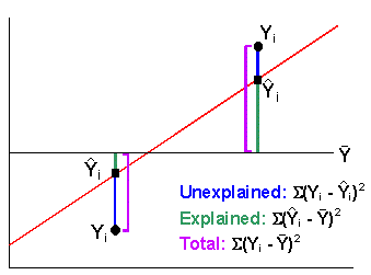
|
In the diagram above, we see that explained
+ unexplained = total.
Therefore, we can calculate the proportion of explained variation to total variation
. This proportion is called the coefficient of determination (![]() ).
This coefficient ranges from 0 to 1; a high
).
This coefficient ranges from 0 to 1; a high ![]() means the line is a good fit, a low
means the line is a good fit, a low ![]() means a poor fit. We interpret
means a poor fit. We interpret ![]() as the percentage of total variation in Y explained by X.
as the percentage of total variation in Y explained by X.
Note: the explained variation is also called the regression sum of squares
(i.e. this is the variation explained by the regression model). The unexplained
variation is also called the residual sum of squares. These terms are
used in the SPSS output.
The final step in evaluating our model is to test significance of ![]() (using the 9 steps for hypothesis testing). The test statistic for the hypothesis
test is F* which compares the explained variation to the unexplained variation.
If a large portion of total variation is explained, F* will be large and we
infer that a significant portion of the variation in Y is explained by X.
(using the 9 steps for hypothesis testing). The test statistic for the hypothesis
test is F* which compares the explained variation to the unexplained variation.
If a large portion of total variation is explained, F* will be large and we
infer that a significant portion of the variation in Y is explained by X.
The following diagram illustrates the concept of this hypothesis test. A full bucket of water represents the total variation in Y. The sponge is the X variable. When the sponge is dipped in the bucket, it absorbs a certain amount of water. The water held by the sponge is the explained variation. The water remaining in the bucket is the unexplained variation.

|
Regression Assumptions
Verifying the assumptions
Some assumptions can be easily verified. For example, you can verify assumption
3 by examining a scatter plot. Other assumptions must be verified by examining
the residual plots (assumptions 4 and 6 - #4 are not covered in this lab). The
remaining assumptions (2, 5 and 7) are required to reduce the computational
load of the regression procedure. These assumptions are very difficult to check
and the researcher must realize that hidden problems may affect the outcome
of the analysis.
The probability distribution, critical values, etc. of the hypothesis test
are detailed in the example.
Before using your model for prediction, you must check for patterns in the residual (unexplained) variation (the difference between the observed and predicted values). By examining the residuals, you may detect patterns or points that influence the fit of the OLS line, or which violate the assumptions of regression. Often these patterns are too subtle to see in a scatter plot.
SPSS calculates
the residual variation for each point in the dataset. For each point, the actual
residual (![]() -
- ![]() )
is converted to a standaridized residual by dividing by the standard error (which
is similar to standard deviation). This process, analogous to producing Z
scores, removes the units of the error term and allows comparison of residuals
between different regression models. The standardized residuals are plotted
on a scatter plot as follows:
)
is converted to a standaridized residual by dividing by the standard error (which
is similar to standard deviation). This process, analogous to producing Z
scores, removes the units of the error term and allows comparison of residuals
between different regression models. The standardized residuals are plotted
on a scatter plot as follows:
The diagram below shows how the errors around the line of best fit are plotted as standardized residuals.
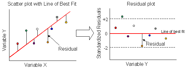
|
How to interpret the residual plot
In the residual plot, the 0 line is the Line of Best Fit (the predicted values).
The residuals show the distance between the predicted values and
observed values. If a residual is close to the 0 line, the distance, or error
is small. If the residual is far from 0, the error between the predicted value
and the observed value is large. Negative residuals mean the equation
over-predicted (the predicted values are higher than the observed values).
Positive residuals mean the equation under-predicted. The ideal
pattern is a random scatter of residuals (positive and negative) between the
two reference lines.
Some problems that you may encounter:
| Outliers: An outlier outside the references lines may reduce the
strength of the regression model (large error = lower | 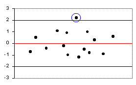
|
| You may also find a residual lying at the far end of the plot, directly
on the 0 line. This outlier has pulled the line of best fit towards it.
This type of outlier may boost the | 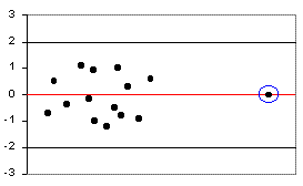
|
| Fan shape: A fan shape in the residuals indicates that the amount of error is not constant along the regression line. At the lower end of the line, the errors are small; at the high end, the errors are large. This pattern is called heteroscedastic (hetero = different, scedastic = scatter). When the error is constant along the regression line, the pattern called homoscedastic (same scatter). You often encounter heteroscedasticity when an additional variable is influencing the relationship. | 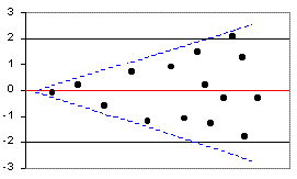
|
| Curve: Residuals in a curve indicate that the relationship between the two variables is not linear. You need to reconsider your variables or conduct non-linear regression analysis (not covered in this lab). | 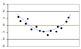
|
| If the | 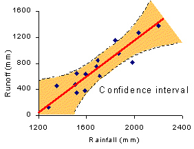
|
| Notice that the confidence interval is curved along the regression line. At the edges of the line, there are few points to support the position of the line. A small change in the position of the line may greatly affect predicted value in these areas (see diagram on right). We are less certain about our estimate so the interval is larger to compensate. In the middle of the line, there are more points to support the position of the line. Therefore, we are more confidence about the position of the line and our interval can be narrower. | 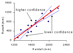
|
There are two formulas for calculating confidence intervals. The choice of formula depends upon the type of dataset you have:

|
| where: S = the standard error of the estimate ( n = the sample size Xi* = the specific X observation used to predict Y Xi = each X observation in the sample |

| (the terms are defined above) |
Why two different formulas? When a dataset contains means, we are more
confident that our sample data represent the population. Therefore, we are more
confident that our line of best fit represents the true relationship between
the variables. We will be more confident about our predictions so our confidence
interval can be narrower.
We will use the rainfall/runoff example to work through 7 Steps to Regression Analysis.
State what type of relationship you expect between the variables and describe the theory supporting this relationship. Identify one variable as dependent and the other as independent. Go to step 2 if you believe the relationship is supported by theory.
Construct a scatter plot to view the relationship between the variables. Calculate the correlation between the variables to assess the strength of the linear association. Go to step 3 if the scatter plot shows a roughly linear relationship, and the correlation analysis indicates a moderate/strong relationship.
| This scatter plot shows a strong positive linear relationship between rainfall and runoff. The correlation (r = 0.91) confirms the direction and strength of the relationship. | 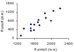
|
Lay out the model you will use (in algebra) and define the X and Y terms. This step may seem redundant in simple regression (with few variables), but it is extremely important when conducting advanced, multi-variate regression analysis.
| where: Y = Runoff (mm) - dependent X = Rainfall (mm) - independent |
Interpret and test the significance of ![]() to determine the performance of the model. Go to step 5 if
to determine the performance of the model. Go to step 5 if ![]() is significant.
is significant.
Hypotheses:
![]() : the independent variable
(rainfall) does not explain the variation in the dependent (runoff) (i.e.
: the independent variable
(rainfall) does not explain the variation in the dependent (runoff) (i.e.
![]() is not different from 0)
is not different from 0)
![]() : the independent variable
explains a significant portion of the variation in the dependent (i.e.
: the independent variable
explains a significant portion of the variation in the dependent (i.e. ![]() is significantly different from 0)
is significantly different from 0)
Significance level: We will use ![]() = 0.05
(95% confidence level)
= 0.05
(95% confidence level)
Probability distribution: The ![]() hypothesis test uses the F probability distribution. The F distribution is
similar to the Chi-square distribution (starts at 0, has only positive values,
and is positively skewed). Click
here for online F Table
hypothesis test uses the F probability distribution. The F distribution is
similar to the Chi-square distribution (starts at 0, has only positive values,
and is positively skewed). Click
here for online F Table
Critical values: Critical F values are based on ![]() and 2 degrees of freedom:
and 2 degrees of freedom:
Test statistic:
The formula for the test statistic is:
![]()
The SPSS output gives the following values:

These formulas are given so that you understand how SPSS calculates the F value. We will use the F value from the SPSS output. For details on conducting the regression and interpreting the output, see the SPSS Help Manual.
Decision rule: The decision rule for this test is: reject ![]() if F* >
if F* > ![]()
In this example, F* (63.47) is greater than ![]() (4.7) so we reject
(4.7) so we reject ![]() . The p-value
calculated by SPSS (p=0.000) confirms this decision.
. The p-value
calculated by SPSS (p=0.000) confirms this decision.
Inference: We infer with 95% confidence that the independent variable
(rainfall) significantly explains the variation in the dependent variable
(runoff) (i.e. our ![]() is significantly
different from 0)
is significantly
different from 0)
Construct a residual plot: the dependent variable on the X-axis, the standardized residuals along the Y-axis. Comment on any problems in the residuals. Go to step 6 if the residuals have a random distribution within the two reference lines. (There are advanced techniques for dealing with heteroscedasticity, autocorrelation, and non-linear relationships but these are not covered in this course.)
| The residual plot shows that the residuals are randomly distributed within the -2, +2 reference lines. This plot indicates that the assumption are probably not violated. | 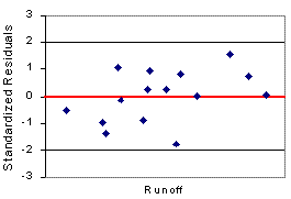
|
Write out the equation using the ![]() and
and ![]() values calculated by SPSS.
Go to step 7 if you are using the equation for estimation purposes.
values calculated by SPSS.
Go to step 7 if you are using the equation for estimation purposes.
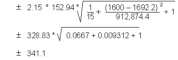
Select the appropriate confidence interval formula (see critieria). Calculate a confidence interval for each predicted value.
 For rainfall of 1,600 mm, the predicted runoff is 607.2 mm. |
|
We express our predicted runoff as follows: 607.2 ![]() 341.1 mm
341.1 mm
By checking our original data, we see that for 1,594 mm
of rainfall (close to 1,600 mm), the observed runoff is 641 mm. Our predicted
value is similar to the observed value and falls within the confidence interval
[266.1 to 948.3].
| Extrapolation The line of best fit should only be used to predict values within or close to those contained in the dataset. Far beyond the dataset, the trend may change and the predictions will be incorrect. The diagram below shows the true relationship between rainfall and runoff. Runoff is less than predicted when rainfall is low, because the water is stored in the soil. Runoff is higher than predicted when rainfall is high, because the soil is saturated and the water runs over the ground surface. | 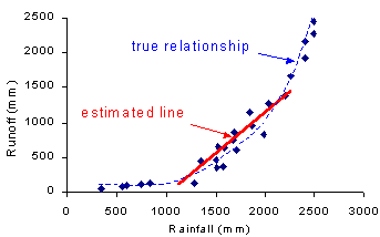
|
Generalization
The regression equation developed from one dataset should not be applied to
data collected in other regions or areas. A regression model developed from
a specific dataset should not be used to generalize about other regions or the
general occurrence of the phenomena. For example, although we find that rainfall
and runoff have a particular relationship in this watershed, we cannot generalize
about rainfall and runoff patterns in all watersheds.
Causation
Although we imply a causal relationship when we use regression, regression analysis
will not prove causality between two variables. Recall that this procedure
is strictly numeric; you may find that two totally unrelated variables give
a significant ![]() . The researcher
must understand the phenomena being researched and the regression procedure
in order to interpret the results appropriately.
. The researcher
must understand the phenomena being researched and the regression procedure
in order to interpret the results appropriately.
| © University of Victoria
2000-2001 Geography 226 - Lab 9 Developed by S. Adams and M. Flaherty Updated: September 29, 2001 |